Documentation

Resensys WebPortal Guide

Thank you for choosing Resensys for your structural health monitoring needs.

If you have any questions that are beyond the scope of these docs, please feel free to email via info@resensys.com.

Account Setup

Follow the steps below to setup your Resensys account.

Before getting started using your wireless monitoring system, be sure you have access to a secure account on the Resensys cloud. If you have not received login credentials, please reach out to the Resensys team via email or call us at (301) 477 3075. From there, we will manage and ensure that your account and device details are properly configured for your specific system.

Once you have recieved your login credentials, navigate to the WebPortal login page to enter your account-specific dashboard.

Personalize First Site

Let's begin by personalizing your first Resensys system site details.

1. Click "Check Data" in the shortcuts to access site.

   

2. Under "Site Selection," select first site from site dropdown list.

   

3. Go up to and select "Site Settings"

   

4. Click the blue "edit" button next to default name to set a unique name for this site.

   

5. Inspect "SenSpot Registrations" for the list of devices, including assigned names, types, status, and IDs.

6. Change site coordinates to update dashboard with site geolocation.

7. Upload a photo for site by clicking on the placeholder image.

8. Toggle the "SenSpot Alerts" tab at the top of site settings; add emails and phone numbers to recieve SenSpot-related alerts.

   

9. Click "SAVE" to apply changes to site settings.

Congratualtions! You have just named, geopositioned, and set alert contacts for your first monitoring system.

Proceed to the next section to learn more about tooling on the portal.

Monitor

The monitor view is intended to provide a overview of different device health metrics and live data streams in a single interface. The interface auto-refreshes to keep health parameters visible and real-time with the option to filter by quantity and/or site.

Overview

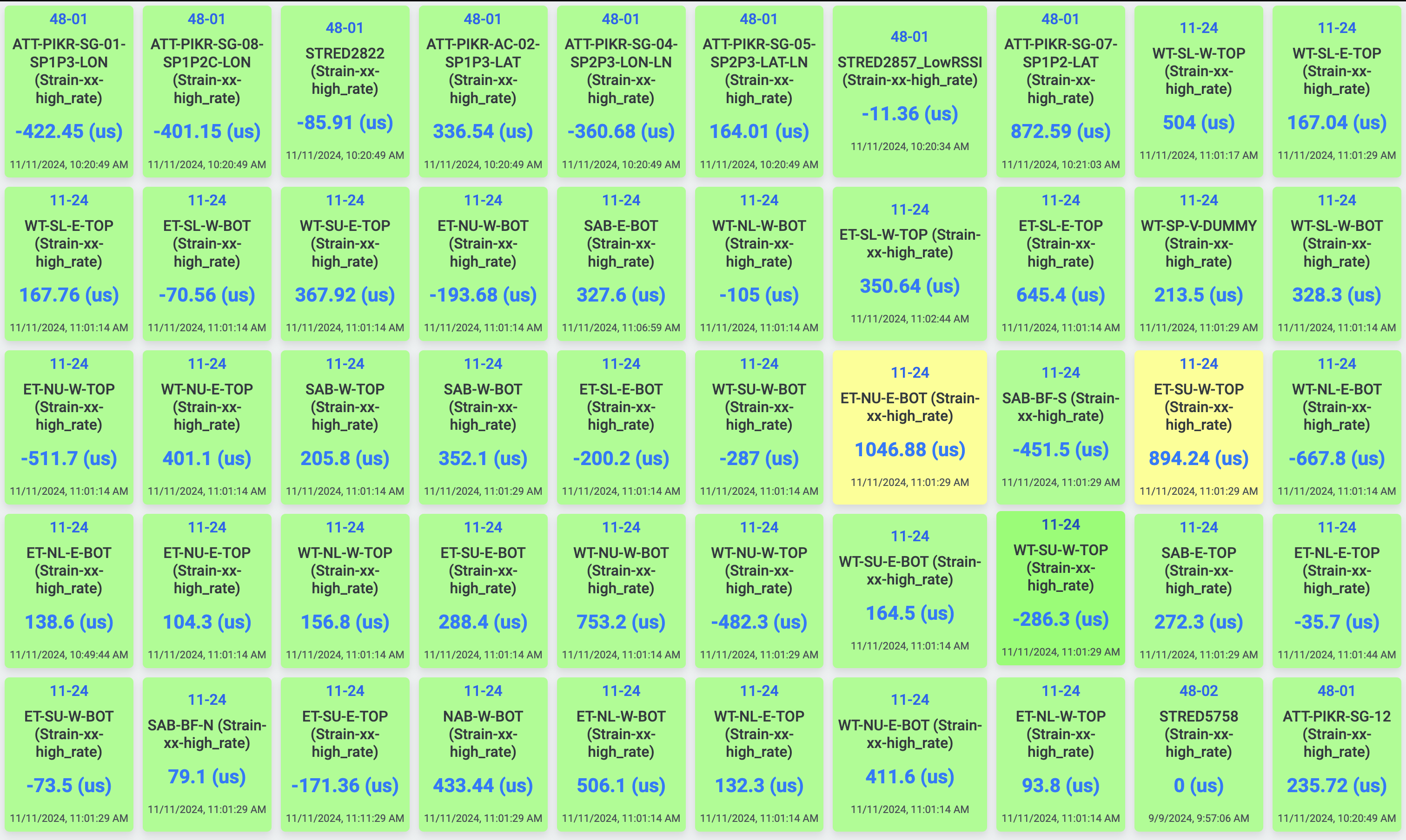
The overview tab allows the user to see the latest readings from one or more quantities across multiple sites. The latest readings can be displayed as cards and/or a 2D layout of the structure with device status indicators color coded. Once loaded in the user's perferred way, the overview will auto refresh every minute with the latest readings, so you do not have to constantly check each data stream manually.

Start by selecting one or more quantities from the list of quantities. Clicking at least one quantity will generate a card grid with the latest readings for any and all devices registered to the user's account. By default, the cards will list the latest readings of all devices across all sites.

If a layout has been applied to one or more sites from the Data Explorer, you can check the box for a subset of sites in the list on the top right of the screen. Selecting a subset of sites will filter the sensor cards with latest readings to devices only registered to those sites and will display a common layout view with the placed SenSpot nodes positioned on the layout.

Card and layout node blinker colors indicate whether the latest reading lies within the normal range, warning range (code yellow), or alarm range (code red). You can tune the alert thresholds per device-quantity pair by opening the device properties form the Data Explorer.

Graph View

In the second tab, you can display the real-time readings of multiple SenSpot data streams against pre-assigned thresholds. The graph tab shows another visual representation of the data as time series plotted against their alert thresholds. This view provides the user with an at-a-glance view of how closely SenSpot measurements are approaching their defined alert thresholds to better plan for operational continuity and safety.

Alert Thresholds

After setting device alert thresholds for available quantities from the Data Explorer, you can display them in real-time with the latest data streams. You can optionally toggle on or off the specific alert thresholds you would like to view for all devices by checking the corresponding boxes in the monitor view tool bar at the bottom of the screen.

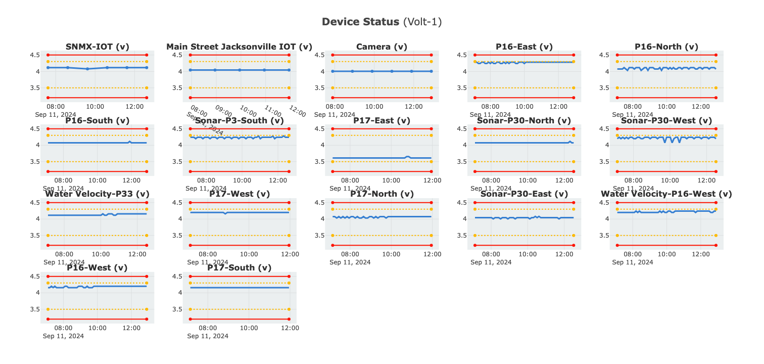
Monitor Duration

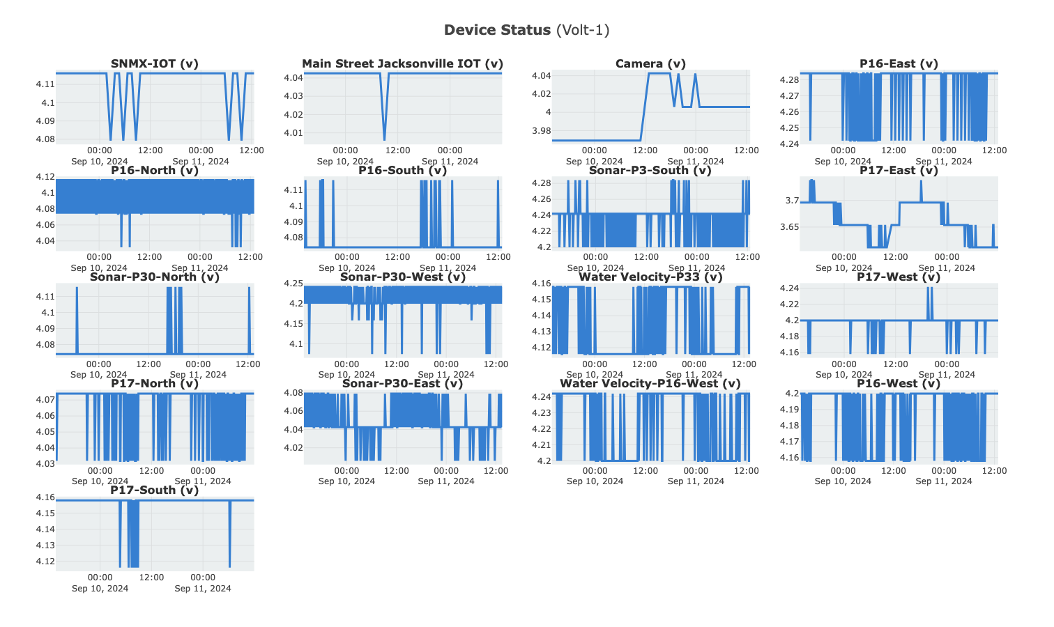
By default, monitoring is shown for a window of the last six hours, but this can be extended to up to 168 hours (1 week). You can set the duration in the field in the montitor view toolbar and click refresh to immediately see changes take effect.

• Range: 1-168 hours.

The following examples show the same data in the last 6 and 48 hours, respectively.

6-hour Monitor View

48-hour Monitor View

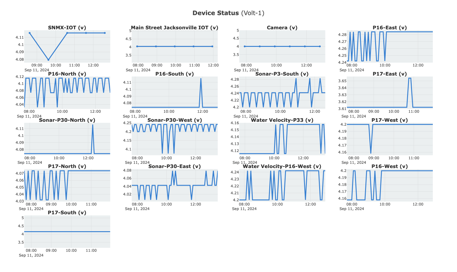
Column Splitting

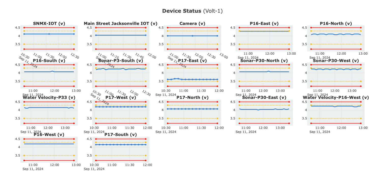
You can display charts on more or less columns depending on the preference of the user. Using more charts allow for a more condensed view of device data streams; whereas, fewer columns provides greater detail.

• Default: 4 columns.

The following examples show the same data for the same duration with 3 and 5 columns, respectively.

3 Column Monitor View

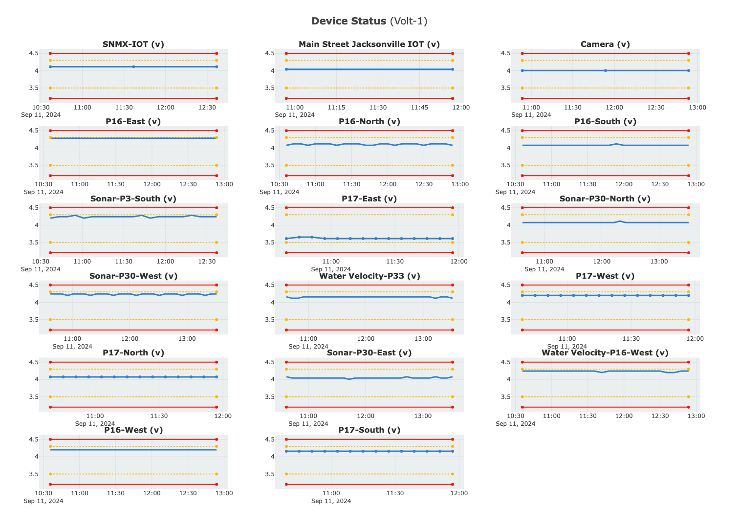
5 Column Monitor View

Quantity Selection

Available and registered device quantities are located in the quanity selection dropup. You can click on the dropup menu and select the quantity you would like to display in the monitor view. Further site-specific filtering is performed by selecting the site from the dropdown at the top of the window.

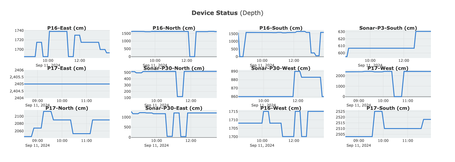
Internal Temperature

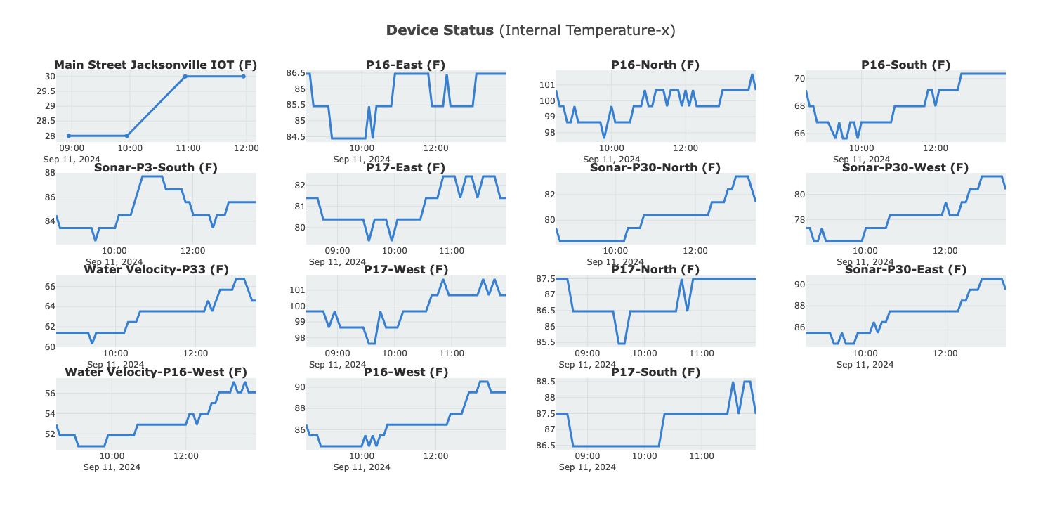
Depth Measurments

Data Explorer

The Data Explorer is the main graphical user interface for exploring and checking SenSpot data remotely from the Resensys WebPortal. It also allows you to directly set device-specific alert thresholds for email and SMS notifications. You can use the Data Explorer to check the status of devices based on their alert status. In the following sections we will provide examples of how to use the Resensys WebPortal in the Data Explorer to get the most out of installed instruments.

Site Selection

Resensys systems are divided into sites and devices. One or more devices can be assigned to a specific site, and these devices are organized into a group on the platform to more easily organize and isolate structures and projects.

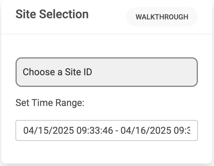
To view the devices for a specific project, click the dropdown displaying "Choose a site ID" and select from the available site IDs.

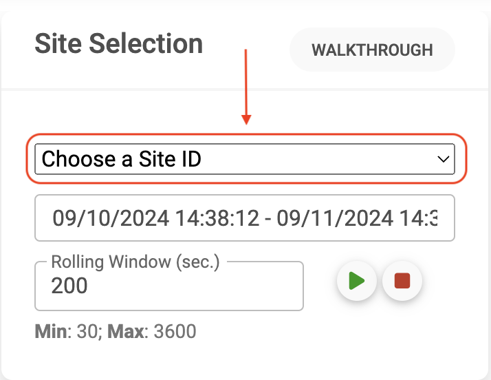
You will be presented with a list of IDs of the form XX-YY. Clicking one of the entries will load the site and all the devices associated with the site or project. You can freely move around different sites by changing the corresponding site ID from the site selection dropdown.

Setting Time Range

All data collected by Resensys SenSpot sensors are represented and stored as measurement time series (e.g. strain, displacement, acceleration). For this purpose, viewing the raw data requires specifying the datetime range. You can use the datetime picker under the site selection field to adjust the window of time of interest. The default time range is the previous 24 hours of data.

Datetime Selection Parts:

1. Quicklinks: Select from a number of common default datetime ranges. Click apply to save changes.
2. Date Range: Click on the start day first, and then click on the end day to set the date range. The days between should be highlighted to indicate a range of dates.
3. Start Time: Set the time to the nearest second on the start date.
4. End Time: Set the time to the nearest second on the end date.
5. Datetime Range Setting: Check the datetime range is set to what you want (local times).

A Note on Timezones:

All dates and times chosen from the datetime picker tool are taken to be local timestamps on your machine's timezone.

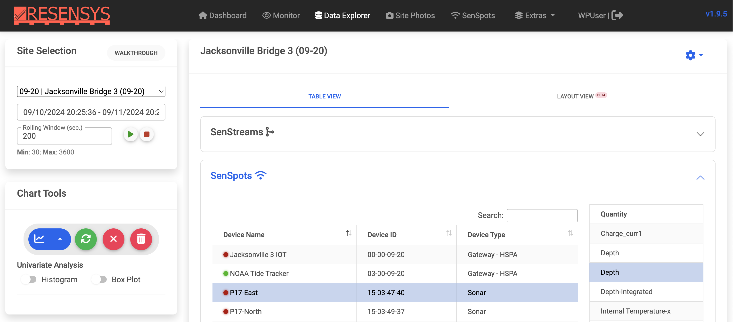
SenSpots List (Table View)

Once a site is selected, the SenSpot list will be populated with devices registered to that site. The default SenSpot list will be displayed in a table view with columns for the device name, device ID, and device type. Beside the device name is a glowing device alert status indicator to easily pin-point devices outside of normal operating ranges. Rows in the device list are selectable for plotting and other charting utilities described in the following sections.

To more easily locate devices by ID or device name, you can use the top search bar. You can also sort by device name, id, and type by clicking the column heading arrows.

Quantity List

Each device reports a collection of quantities. In order to view the data from these reported quantities, you should first select a device from the device list, and the quantity list to the right of the device list will update to reflect the selected device's quantities.

Basic Plotting

The basic operation of the Data Explorer includes adding, removing, and refreshing time series on a main or primary chart. To do this, you use the four button just under the Chart Tools section in the left pane of the UI. There are four button controls for basic plotting (left to right):

1. Add Chart (blue): Uses the selected device and quantity from the device and quantity lists to add one or more time series of collected SenSpot to the main chart within the specified datetime range.
2. Refresh (green): Adjusts or updates the main chart to reflected an updated time range or chart option (discussed in following sections).
3. Clear Chart (red): Clears only the content of the main chart from the UI.
4. Clear All (red): Clears the main chart and any accessory charts/analyses.

Note: by clicking the "Clear Chart" or "Clear All" buttons, you are not and cannot delete data from storage on your account. All historical records are securely and durably stored on the Resensys cloud.

Chart Tools

Univariate Statistics

You can get the univariate statistics for up to two data streams by checking either the histogram or box plot options below the basic plotting utilities. You can view the distribution of data in a histogram and/or box plot and get a summary of the single-variable statistics of the time series displayed in the main chart. You can also adjust the time range and refresh all plots to update the summary statistics.

Spectrum Analysis

Spectral analysis is used to characterize the response of a structure in the frequency domain. Using techniques like the Fast Fourier Transform (FFT) one can determine the fundamental frequency of vibration at a particular point on a structure. One can use the built-in spectral analysis tool within the portal to compute the FFT on one or multiple triggered accelerometer events and track changes or shifts in frequency responses over time.

To use the spectrum analysis tool, you should first plot a time series on the main chart (e.g. HPA-Z for an accelerometer SenSpot). Next, click the compute FFT button within the spectrum analysis tool in the left chart tool pane. A new chart with the input signal and the output FFT will be displayed side-by-side. These results can be saved to an image as a PNG for easy reporting or expored directly to a file for further analysis and logging.

Linear Regression

To quantify the relationship between a pair of SenSpot data streams, one can perform a simple linear regression to characterize any linear dependencies. This can be useful for evaluating performance of bridge members and detect any non-linearities between adjacent sensors.

To get started, scroll down to the linear regression tool in the left chart tool pane. Now, you can select a device from the device list and a quantity. With a device-quantity pair selected, you can click the + button to load the pair into the linear regression tool. Load two pairs and click the calculate button to run the analysis. The resulting analysis can be saved as an image to a .png or as a flat file for further analysis.

Rainflow Counting Analysis

Rainflow analysis is a method used in fatigue analysis to characterize and count the cycles of stress or strain in a time-series data set. It is used in conjunction with strain gauge SenSpots to ascertain the half cycles of stress attached to a bridge member.

You can run a rainflow counting analysis by importing the "Strain-xx-high_rate" quantity for a given strain gauge into the primary input field (red outline). Then set the bin size, which specifies the range of stress in ksi (typically 0.01), and the modulus of elasticity (29000 ksi for steel). Once the primary field, bin size, and modulus are supplied, click run to run the analysis. The output of the analysis can be saved as an image to be included in reporting, and the data and counts from the rainflow counting can be stored to a file.

Plotting Options

There are several plotting options/function available to modify the action of the Add Chart button. If you click the dropup menu button to the right the Add Chart button, there are several options available:

1. Remove Average: Calculates the average of a raw SenSpot timeseries and subtracts from all raw calibrated measurements. This can be used to remove the effect of differing offsets for data streams between devices.
2. Median Filter: Used to apply a rolling median to the time series to smooth the output. This can be used to remove or ignore outliers from a raw output.
3. Show Alert Levels: Once alert levels are set for a device-quantity pair, you can view the alert levels simultaneously with the raw SenSpot data.
4. UTC Timestamps: Toggle on or off UTC timestamps. The default timestamps are local to the timezone of your machine, but you can use this option to use a more consistent and universal time reference.
5. Downsample Interval: A set of options to reduce the output of data in the main chart (e.g. M1 = "1 minute intervals"). This can be helpful if trying to visualize long-term trends over several months but only need to track general trends.

Importantly, each of the plotting options are intended to be independent of each other. This means that they can be independently toggled on or off and multiple plotting option function can be applied to the output of timeseries on the main chart.

Additionally, the plotting options are persistent across all time series added to the main chart. For example, if you toggle the "Remove Average" option, all subsequent plots on the main chart will be rendered with all time series' averages removed until the option is toggled off.

Device Properties

Each device has a set of device properties which can be accessed by double-clicking the device row from the device list in the Data Explorer. These are separated into General, Calibration, Notes, and Alerts. The following details what each tab/section of device properties describes:

1. General: Specifies the name, site ID, device ID, device type, and activation status of a SenSpot. The activation status informs whether the device should appear in the device list when selecting a site.
2. Calibration: A table of calibration coefficients and offset for each quantity of the selected device. Calibration coefficients should not be changed, but offsets can be set to shift time series up or down (e.g. to zero readings).
3. Notes: A textbox to leave device-specific notes for you and your colleagues.
4. Alerts: A table of alert thresholds defined for each quantity registered to the selected device. More details in the following section.

Device Alert Levels

Setting device thresholds for email and SMS notifications is handled within a device's specific device properties. The alert scheme used by Resensys consists of two code yellow ("warning") and two code red ("alarm") levels. These four thresholds can be defined and set on a per device-quantity basis and adjusted as needed. Double click a device from the device list to get started.

Setting Threshold

Start by setting the thresholds for ALARM_LOW, WARNING_LOW, WARNING_HIGH, and ALARM_HIGH for one or more quantities in device properties. You can set the status to the off/inactive position to ingore reporting these quantities. Be sure that alert levels are set such that

ALARM_LOW < WARNING_LOW < WARNING_HIGH < ALARM_HIGH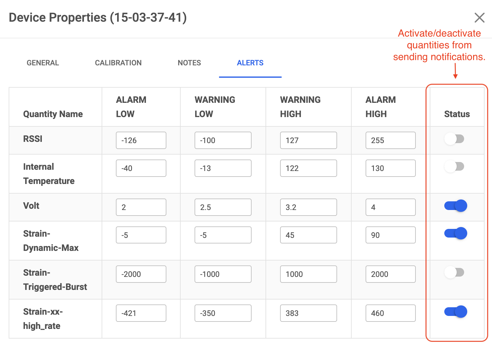

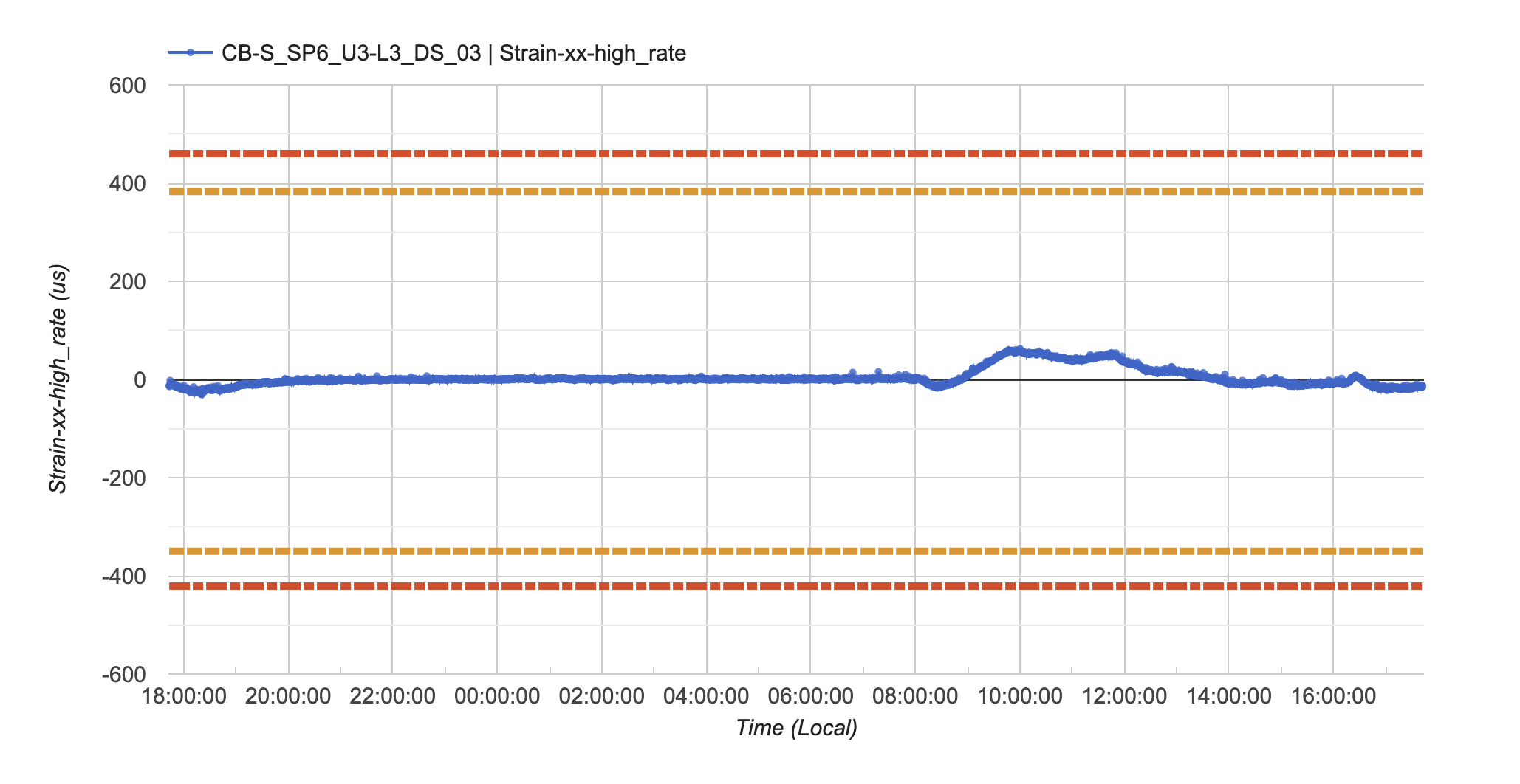
Displaying Threshold

You can verify that alert threshold are set appropriately by plotting them along with real SenSpot data.

When setting alert thresholds, we recommend toggling the Show Alert Levels plotting option to confirm appropriate levels have been set. Enabling this option will produce chart with the alert levels, and an example is shown below.

SenStreams

In many cases, the raw data transmitted by SenSpots (sensor nodes) do not directly correspond to the specific fields or parameters needed for in-depth structural analysis. For instance, while strain gauges attached to a steel bridge may measure strain in units of microstrain, engineers may be more interested in the stress acting on the structure, which is expressed in different units and derived from strain measurements.

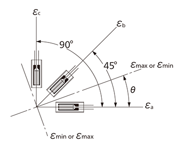
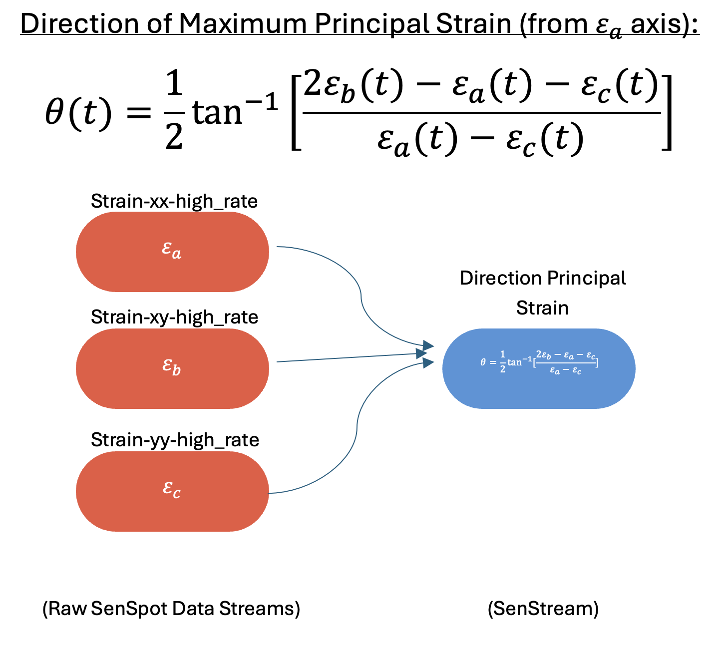
Additionally, it is often necessary to combine multiple data streams from different SenSpots or monitoring locations. For example, rather than analyzing individual temperature readings from each SenSpot, you might want to compute a temperature gradient across the entire structure to assess how temperature changes over time and space. You may also decide to combine all the strain channels of a rectangular rosette strain gauge to output the direction of principle strain (see example right).

To address these needs, we introduce SenStreams. A SenStream is a computed field that applies a custom formula or transformation to one or more raw SenSpot inputs, producing a new, tailored data stream. This new stream can represent quantities like stress derived from strain, temperature gradients across different points, or other combinations of raw data that are more relevant for advanced analysis.

In essence, SenStreams act as a tertiary compute layer on top of your structure, allowing for the creation of complex, real-time data models by transforming and combining raw sensor data. This enables more precise monitoring, modeling, and decision-making based on the specific needs of your structural health analysis.

To get started, locate the SenStream dropdown component at the top of the Data Explorer. At the bottom, click the "Show Tools" button.

Layout View

2D Layout View

As an alternative to the table view of device list, you can set up a layout view of a structure by uploading structural drawings for a specific site. In the layout view of a site, SenSpot nodes are placed directly on the engineering drawings of the structure, are selectable, and interactive. Similar to the table view, glowing indicators both mark the locations of SenSpots on the structure and their associated alert state in relation to set device alert thresholds.

To upload a layout, we recommend that you first convert the drawing of the structure to a .png or equivalent file format. If you face any difficulties uploading, please reach out to the Resensys team at info@resensys.com.

The same functionality from the table view including access to device properties and plotting is present in the layout view.

3D Layout View

With 3D layouts, you can visualize an entire structural asset in 3D and directly attach SenSpot nodes directly to the structure. You can also leave notes for colleagues about locations of interest or locations to inspect more closely by attaching annotations. Previous inspection reports can be attached directly to the structure with PDF upload structural markers.

The following video demonstrates the basic functionality and interactions with 3D models on the Resensys web platform.

ReportGen

The ReportGen tool is designed to address the what, when, where, and how of large-scale structural health monitoring and reporting. It provides a highly extensible, schedulable, and sharable reporting service that you can use across multiple monitoring projects.

With ReportGen, you can create stored templates of relevant data from one or more sites, organize multiple panel types into a custom layout, and even schedule automated report generation. These scheduled reports can be delivered directly to specified email recipients on a daily or weekly basis. Whether you want a one-time inspection report or a regularly updated report on critical infrastructure, ReportGen allows you to configure and automate the data extraction and presentation process.

The key advantages of ReportGen include the ability to combine data extracts from multiple sites into a single digital report, exporting data in multiple file formats (e.g., CSV, Excel, and more), and extensive layout customization options that let you highlight exactly what matters most to your colleagues or stakeholders.

Getting Started

Before creating your first report, it helps to understand how the tool is structured. ReportGen abstracts the creation of data reports into two main entities: templates and panels. Every report has at least one template, and each template can have one or more panels.

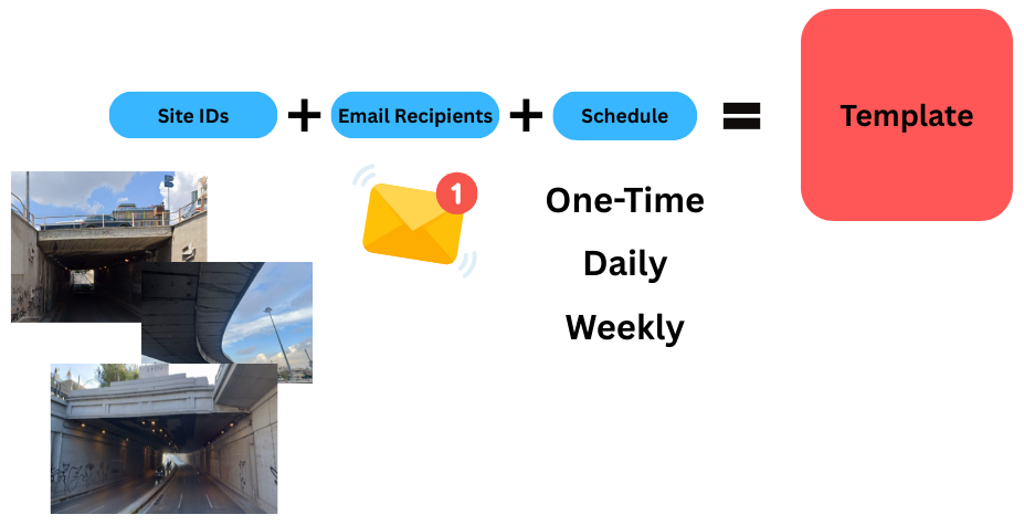
When you create a new report, you begin by adding a template. You can give this template a name, associate one or more sites by their site IDs, choose a schedule (one-time, daily, or weekly), and provide one or more email addresses to receive automatically generated reports. It’s perfectly acceptable to create multiple templates to summarize data under different contexts (for example, summarizing daily temperature trends vs. weekly alert thresholds).

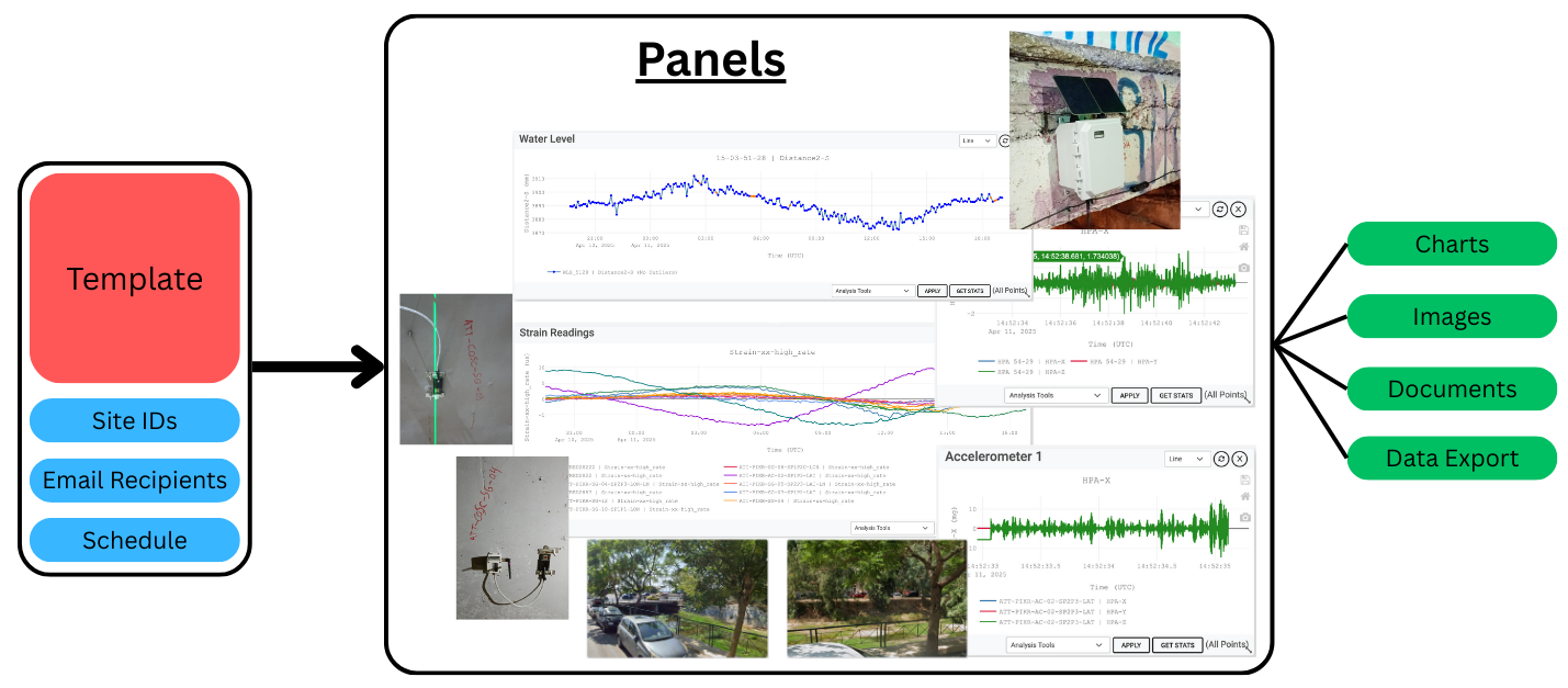
A template organizes the final report into panels, each of which focuses on a particular data element or visual resource. These panels can contain time series charts, uploaded images, or PDF documents, allowing you to combine sensor data with external references or supporting documentation.

Navigation

The ReportGen interface is divided into two main sections:

• Template Creator/Selector (Left Sidebar): Here, you define or select a report template, specify its sites, set an optional schedule for automatic generation, and determine who receives the final reports by email. You can create a new template by clicking + New Template at the top of the sidebar.
• Report Grid Area (Right): Once you select or create a template, the right side of the screen shows the panels you have added to that template. This area is where you add new panels, arrange them, and access data export options.

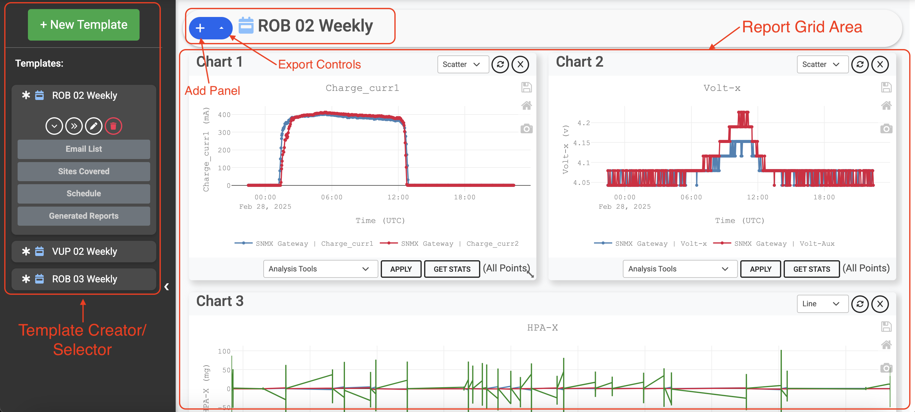
Each template in the left sidebar has an icon indicating its schedule interval: a lightning bolt for one-time reports, a calendar-day icon for daily reports, and a calendar-week icon for weekly reports. You can toggle the sidebar’s visibility using the arrow icon if you need more space to view or edit the report’s panels.

In the upper area of the report grid, you’ll see the selected report template’s name, the New Panel button , and a dropdown menu for data extraction and template management. Any modifications you make—such as adding panels, changing their layout, or updating panel parameters—can be saved by choosing Save Report in that dropdown.

Panels

Panels are the individual elements added to a report template to convey key information about your site(s). You can drag and resize them to highlight important metrics, images, or documents. Currently, ReportGen supports three main panel types: Time Series, Image, and PDF Upload.

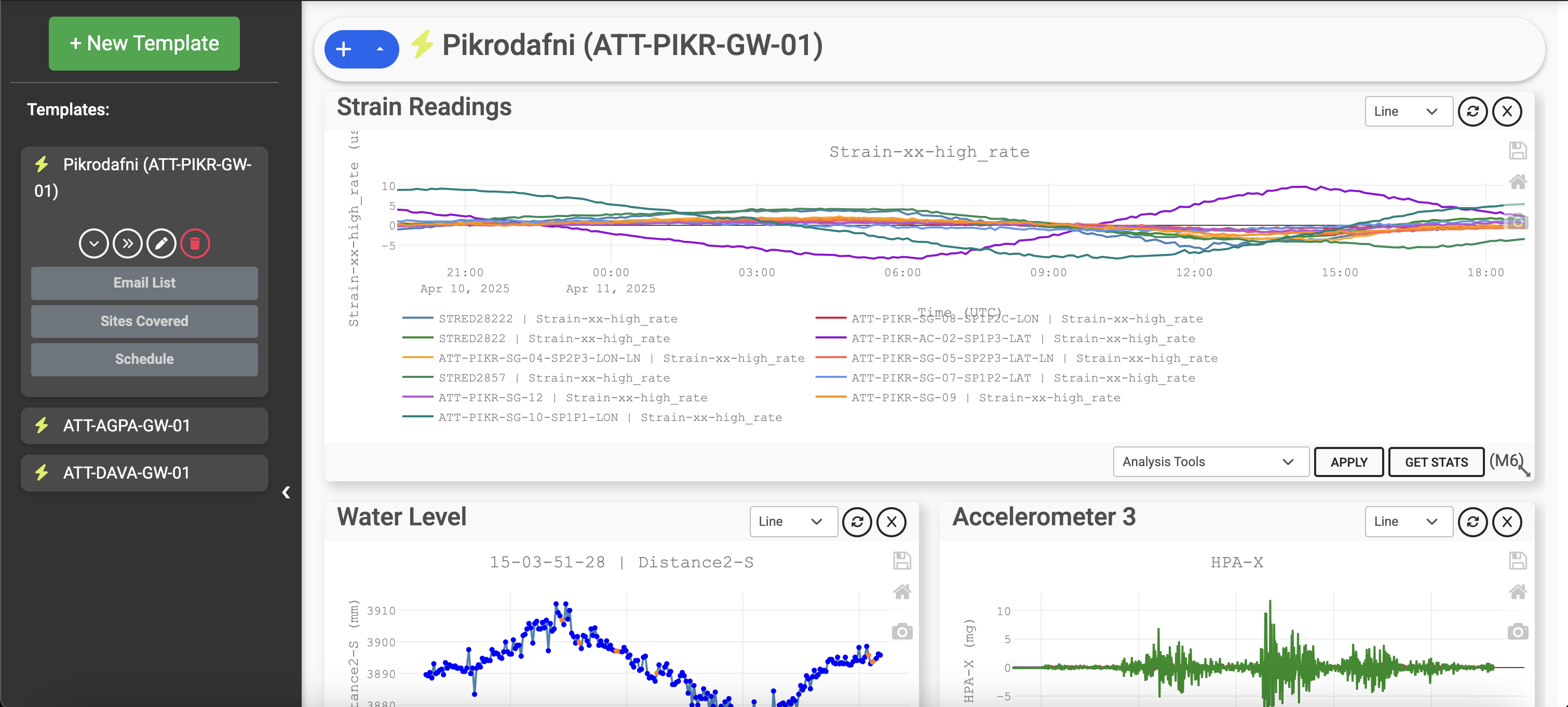
Time Series

A Time Series panel displays sensor data points over time. You can select and combine multiple data streams from one or more devices across the sites specified in your template. Each chart can be independently configured to show line, scatter, or bar charts, and you can set different down sampling intervals for more efficient loading. You can also overlay alert thresholds (previously set in the Data Explorer) to show if any sensor readings exceed certain limits.

Image

An Image panel allows you to upload PNG or JPEG files directly into your report. This feature is especially useful for adding photos from an installation site, capturing the orientation or placement of sensors, or supplementing time series data with visual inspection images and annotated drawings.

PDF Upload

With a PDF Upload panel, you can embed an entire PDF document directly into your report. This is handy for providing additional supporting documents—such as previous inspection records or third-party analysis—without having to copy or reproduce the content elsewhere. Including these reference PDFs in your report template ensures that all relevant information is kept together in a single, cloud-accessible platform.

Important: Remember to click the Save Report button (in the dropdown at the top of the report grid area) to save any changes you make to your panels.

Exporting Report Data

There are two primary methods for exporting data from your reports:

1. Individual Chart Export: Any Time Series panel can be exported to a separate CSV file containing just the sensor data traces shown in that chart. This is quick if you only need a specific subset of data.
2. Global Export: In the top dropdown of the report grid area, you can choose multiple export options to extract data from all panels in the selected template:
   • File Types: Export data to CSV, XML, TXT, or XLSX.
   • Combining Traces: Export all traces into individual files, one combined file, or by chart. You can also toggle Interpolate Gaps to fill in missing points using linear interpolation.
   • Digits of Precision: Specify how many decimal places you want (1–6).
   • Export Data: Initiates the data extraction from the Resensys cloud for all traces in the template with your chosen export settings.

Clicking Save Report in the same dropdown will store your current template configuration in the cloud environment so you can revisit it or reuse it later.

Template Layout

Each panel element within a template can be sized and positioned independently to emphasize certain visuals or datasets. You can click and drag the header of a panel to move it to a different location, or grab the lower right corner to resize it vertically or horizontally. This flexibility lets you tailor the report layout according to the relative importance of specific data or images.

Because of this adjustable layout, it’s straightforward to build dashboards that highlight critical information first or group panels based on thematic or functional similarities. For example, you might cluster all Time Series panels together for quick data analysis, while placing visual references (images or PDFs) at the end of the report.

Analytics and Chart Panel Tools

Each Time Series chart panel includes a suite of analytical tools to help you preprocess or analyze your data. These tools can be used individually or stacked together in sequence, and ReportGen will remember the order they are applied, reapplying them for any auto-generated, scheduled reports. Some of the tools include:

• Remove Average: Subtracts the average from each trace.


• Rolling Average: Applies a smoothing filter by computing a moving average over a user-defined window.


• Extract Trend: Calculates and displays a linear trend on top of the original dataset.
• Remove Linear/Polynomial Trend: Fits a linear or polynomial trend of degree p and subtracts it from your data.


• Remove Outliers: Automatically excludes data points that lie beyond three standard deviations using a Median Absolute Deviation (MAD) calculation.


• Show Spikes: Highlights all points outside three standard deviations of the mean.
• Interpolate Gaps: Fills in missing data points via linear interpolation.


• First Difference: Transforms the time series by taking the difference between consecutive data points.


• Simple STDEV Threshold: Identifies points that lie outside a specified number of standard deviations.
• Detect Outliers: Uses MAD-based detection in a rolling window to find outlier points in each trace.


• FFT: Performs a Fast Fourier Transform on the selected time series with optional high-pass or low-pass cutoff filters.


• Numerical Integration: Integrates the time series data, which can be especially helpful for converting accelerometer data to velocity or displacement for additional analyses.

By applying these transformations, you can save a preprocessed data set in your report, enabling recipients to focus on the most pertinent insights without having to re-process the raw data. ReportGen’s ability to automate the reapplication of these transforms for scheduled reports is a powerful way to maintain consistency in your analyses over time.

Alerting

Alerting is a central component for most structural health monitoring projects. The Resensys WebPortal allows users to configure two general alert types: synchronous and asynchronous. Read on to learn how you can use Resensys alerting for your strucutral health monitoring application.

Synchronous Alerts (Real-Time):

Synchronous alerts are closer to real-time and a triggered as soon as a SeniMax site ID connects to dump data and are configured and managed from the "Alerting" tab of the Resensys WebPortal. A synchronous alert treats all SenSpot measurements as equally likely to trigger an alerting condition, where each measurement is streamed chronologically and checked individually. You will want to use a synchronous alert whenever you want to minimize the delay between an alerting condition and a notification being sent to recipients. With synchronous alerting, you can also tune the sensitivity for sending notifications by adjusting the Critical Points parameter for each record. The number of critical points specifies how many consecutive measurements must satisify a triggering condition before an notification is sent--a larger value means the alerting is less sensitive to outliers or short-lived spikes in data.

Asynchronous Alerts (Legacy):

Unlike synchronous alerts, asynchronous alerts are not triggered for processing exactly when data first becomes available and is dumped by a SeniMax. Instead, alert condition detection occurs in cycles, where alert records specify how and over what duration to process a whole time series. Asynchronous alerting takes data from the past three (3) to twenty-four (24) hours and performs an advanced check against a four-threshold alerting scheme: alarm low, warning low, warning high, and alarm high. The latter four thresholds are configured per quantity per unique device ID, and the user can access and configure these alert thresholds from the Data Explorer tab and opening a device's device properties.

In general, asynchronous alerting can take up to 20 minutes to process and send an notification message; whereas, synchronous alerting should be sent consistently within 2 minutes. The content of synchronous alerts is simple but timely, while the content of asynchronous alerts is more visual with some delay.

In the following sections, we describe how to configure the different classes of synchrounous alerts including creating new alert records, updating existing records, deleting records, and activating/deactivating specific alert records for notifications.

Alert Classes

Synchronous alerting performs simple numerical comparisons between a preassigned threshold and each measurement being streamed into the alerting system. For this purpose, there are two basic classes of synchronous alerts that can be configured by the user: ABOVE and BELOW. For example, if you want to create a check whenever a wireless Strain Gauge SenSpot's strain reading exceeds 100 microstrain, you can create an alert of type ABOVE and set the threshold to 100 for the field "Strain-xx-high_rate". As another example, should you want to be notified whenever the battery voltage in a tiltmeter drops below 2.7 volts consistently, you can configure an alert of type BELOW and set the threshold to 2.7 for the quantity "Volt".

Alert records of either class are processed and handled independently, meaning that the processing and detection of an alerting condition on one record is completely isolated from another record. This feature allows for stable at-scale alerting for any number of devices and sites.

Additionally, alerts of type ABOVE only check then the configured quantity rises above the threshold, but does not check when it drops below--similarly, for the alerts of class BELOW.

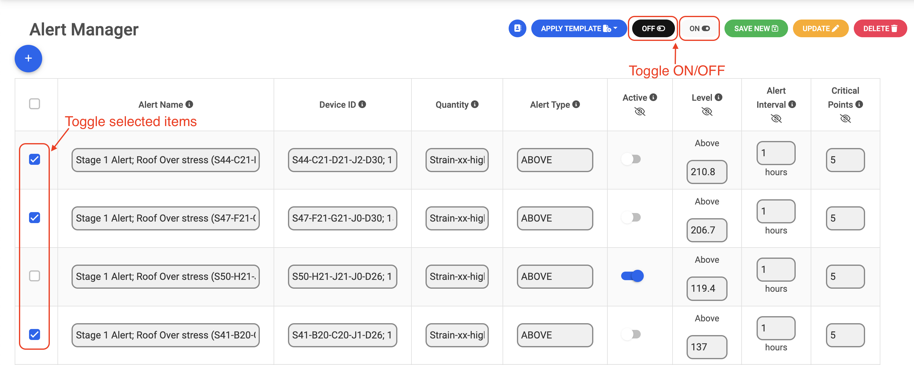
Create New Alert

To create a new alert, you can start by selecting the "+" sign in the top left labeled "New Alert". A new row will be generated in the main alert records table. The following explains in more detail each of the relevant fields that should be filled in to complete the alert record setting:

1. Alert Name: Provide a descriptive name for the alert that will be sent in the notification and can be used to distinguish from other alerting checks.
2. Device ID: Locate and select the device ID by assigned title; the data streams of this selected device will be used for alerting.
3. Quantity: Select the quantity reported by the listed device for which alert checks will be made (e.g. select "Strain-xx-high_rate" to check level of strain readings).
4. Alert Type: Choose type ABOVE or BELOW to check if real-time readings are above or below the define threshold level, respectively.
5. Active: Toggle to the on position, and you will recieve notification; toggling off will save the settings of the alert record, but no notifications will be sent.
6. Level: Set the numerical thresholds specific to the alert record according to the alert class (e.g. ABOVE or BELOW).
7. Alert Interval: Specify the duration between notification to be sent to recipients while the alert condition is true. For example, setting the alert interval to 12 hours will result in notifications being sent every 12 hours while the relevant alert condition is true for at least the last 12 hours. The system will continue to send notifications until the alert threshold is adjusted or the measurements no longer satisfy the alert triggering condition.
8. Critical Points: The number of consecutive points that satisfy an alerting condition needed to send a notification. Setting the criticial points for an ABOVE alert record with value 5 means that the data stream for alerting will need to wait for 5 consecutive points to be above the set threshold before sending an email or text message. This parameter is useful for tuning the sensitivity of the alert and for filtering out pointwise outliers or spikes in a data stream.

Once alert records are set, check the boxes in the first column and click "SAVE NEW" to add the new records to your account. You will recieve a notification when the alert records have been successfully applied to the account.

Update Alert Record

To update one or more alert records, you can modify a records' fields or select the checkbox for each record to be updated. Once all the fields to be updated have been adjusted and the checkboxes selected for update, click the "UPDATE" button in the top right ribbon to apply the changes.

You will recieve an notification that the update command was sent to apply the changes for the selected records.

Delete Alert Record

To delete one or more records, select a subset of records' checkboxes and click the "DELETE" button in the top right ribbon. You will recieve a notification that the records were successfully removed from your accounts.

Activate/Deactivate Alerts

The user can optionally turn on or off alert records for notifications. To do this, select a subset of alert records by checking their checkboxes, then click the "ON" or "OFF" button in the top right ribbon to toggle them off. Click "UPDATE" to apply the changes to your account.

Remote Control

Use the remote control to adjust the transmission interval of a remote SeniMax. Placing a SeniMax into fast sampling can help those in the field conduct inspection with higher SenSpot sampling. Setting sites in fast-sampling also aids in conducting live load tests.

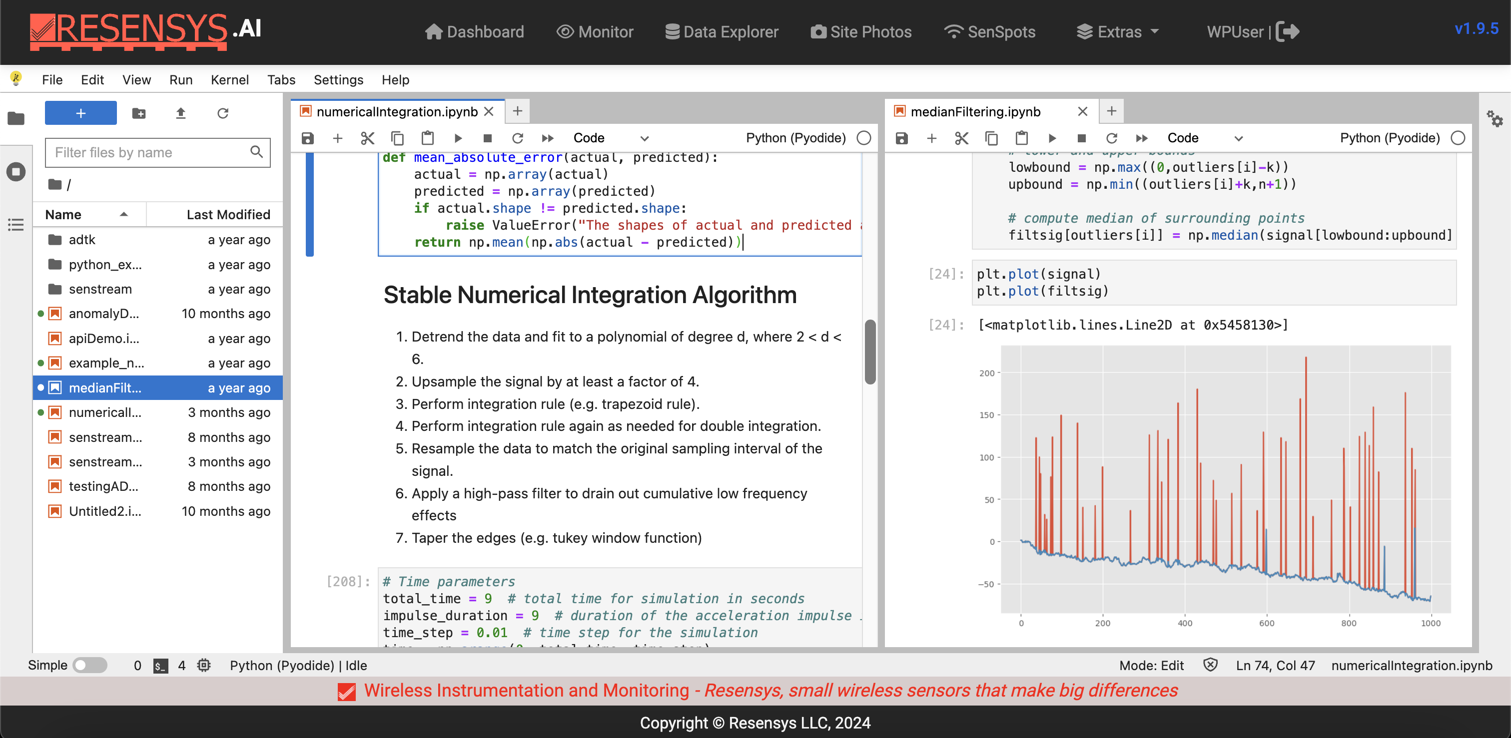
JupyterLite

Perform more customized data analyses directly from the portal in a browser-native Python3 environment. The JupyterLite interface presents a user-friendly interface and a lightweight python environment based on Piodide with access to some of the most commonly used libraries and packages using for data analysis (e.g numpy, scipy, pandas, etc.).

SenSpot Quantities

General Quantities

• Volt: Voltage measurement of primary Lithium battery within each SenSpot.
• Internal Temperature: Measured in degrees Celsius or Fahrenheit, the internal temperature is reported from an on-board temperature sensor within each SenSpot and is calibrated to temperatures between -13 degrees F to 122 degrees F. This temperature measurement is collected at the wireless transmitter and not the transducer.
• RSSI (Received Signal Strength Intensity): A measure of the relative signal strength intensity of the radio communication between a SenSpot and a gateway. This quantity can be used to determine if and when a SenSpot synchronizes with a SeniMax gateway and is a proxy for the relative distance to the gateway. Values closer to zero indicate a stronger signal (i.e. -30 to -10 dBm) whereas values closer to -80 dBm indicate a very weak signal. Absent or partial desynchronization with a gateway will have a default RSSI value of -127 dBm.
  • Full scale: -127 to 0 dBm

Strain Gauge SenSpot

• Strain-xx-high_rate: High-rate data stream for axial strain measured in microstrain. In normal sampling, strain measurements are performed once every fifteen (15) seconds but can be increased to two samples per second in 30-seconds fast sampling mode.
• Strain-Triggered-Burst: Data collected during burst mode of SenSpot in which the absolute change in strain measurements exceeds a set threshold in microstrain. These axial strain gauges constantly record a moving average of strain in background at 40 samples per seconds, and report data in burst mode if any of the aforementioned events are triggered. Data for each burst event records data for one second before the triggered threshold and eight seconds after.
• InfoField3: A quantity that indicates the threshold and the sampling interval of the triggering function. It is calculated in the following way:
  • InfoField3 = threshold_raw_value * 256 + sampling_interval
  • Actual threshold in µS = threshold_raw_value*4*quanity_coefficient (in the Portal)
    • E.g., if “Info Field 3” reads 537 = 256*2 + 25, it means the threshold is 8*coefficient and the sampling interval is 25ms.
  • A threshold raw value of 255 will disable the event detecting function.

Accelerometer SenSpot

• HPA-X: Measurement of acceleration along the X-axis of the device measured in mg (one thousandth the magnitude of acceleration due to gravity on Earth, about 9.81 m/s/s); the full range in +/- 2g.
• HPA-Y: Measurement of acceleration along the Y-axis of the device measured in mg (one thousandth the magnitude of acceleration due to gravity on Earth, about 9.81 m/s/s); the full range in +/- 2g.
• HPA-Z: Measurement of acceleration along the Z-axis of the device measured in mg (one thousandth the magnitude of acceleration due to gravity on Earth, about 9.81 m/s/s); the full range in +/- 2g.
• InfoField1: Data stream showing the current magnitude of the triggering acceleration threshold in mg for all three axes (HPA-X,Y, and Z).
• InfoField2: A measure of the on-board memory usage from detected triggered events. A value of 0 indicates that the memory is empty while a value of 255 corresponds to memory being full. When the memory is full, the accelerometer will cease collecting more event- triggered data until it is able to transmit some of its data to a SeniMax gateway.

Water Level SenSpot

• Distance1-S: Measures the calibrated distance in feet based on calculated time delay between sending and receiving ultrasonic pulse from sensing element.
• Distance2-S: Measures the calibrated distance in mm based on calculated time delay between sending and receiving ultrasonic pulse from sensing element.

SeniMax Gateway

• Charge_curr1: Data stream reporting the charge current in battery corresponding to volt-x from the solar redundant power supply measured in milliamps.
• Charge_curr2: Data stream reporting the charge current in battery corresponding to volt- aux from the solar redundant power supply measured in milliamps.
• RSSI-x: A measure of the relative signal strength intensity of the radio communication between the SeniMax gateway and ATT cell towers. Values close to zero indicate poor, weak or no cell signal (i.e. 0 to 10 dBm) whereas values closer to 30 dBm indicate a very strong and reliable signal.
  • Full scale: 0 to 31 dBm
• Volt: In the context of the SeniMax gateway, “Volt” records each time that the device successfully connects and receives a response from a server through the cellular network. In this way, the raw value of this quantity yields no information; however, the timestamp can be used to determine whether the device is operating and in what sampling mode the device is running (i.e. normal- or fast-sampling mode).
• Volt-x: Measures the actual voltage of one of the two rechargeable 18650 Li-ion batteries in SeniMax gateway. The operating range of these batteries is 3.6 to 4.1 V with the battery being 90% charged at 4.0 V.
• Volt-aux: Measures the voltage of other rechargeable Li-ion batteries in SeniMax gateway.

FAQ

Changelog

See what's new added, changed, fixed, improved or updated in the latest versions.

Version 1.4 (27 February, 2025)

• New ReportGen feature is introduced to help users automate data extractions and file storage. Create fully customizable reports with charts, shared image files, and PDF uploads to share with colleagues. More details in the "ReportGen" section in these docs.
• Updated dashboard page to summarize sites on map view visualize the site status, check the latest alert logs, and inspect new reports generated.
• Cleaned up the layout of the Data Explorer to simplify the interface for viewing and using accompanying chart tools.
• Introduced 3D layout view for limited users for placing sensor nodes, uploading files, and annotating directly on point clouds of a structural asset. To learn more, you can reach out to info@resensys.com.

Version 1.3 (18 November, 2024)

• Added descriptions for the most common quantities reported by different Resensys devices in the "SenSpot Quantities" section--new quantities for device types to be added.

Version 1.2 (11 November, 2024)

• Added information about most common quantities reported by devices.
• Included new documentation for recent changes to monitor view to include real-time sensor cards with latest readings and how to load a real-time layout overview for one or more sites.
• Documentation for Resensys Alerting tool added: asynchronous vs. synchronous alerting.
• Creating, updating, and deleting synchronous alerts is explained in the "Alerting" section.

Version 1.1 (11 September, 2024)

• Included additional details about the use of senstreams and setting/viewing device alert thresholds.
• Documentation for the use of the Monitor tool added.

Version 1.0 (18 December, 2023)

• Initial release.